LVQ压缩算法论文阅读笔记-Similarity Search in the Blink of an Eye with Compressed Indices
LVQ压缩算法论文阅读笔记-Similarity Search in the Blink of an Eye with Compressed Indices
Ding Ning论文简介
Similarity Search in the Blink of an Eye with Compressed Indices 是一篇 Intel Labs 发表于 2023 年 VLDB 的论文。
论文贡献
1、提出了一种新的压缩算法,名为 Locally-adaptive Vector Quantization (LVQ), LVQ 是在 标量量化 Scalar quantization 的基础上进行局部优化的压缩算法,通过更低的压缩率、实现了更少的精度损失,并提供了两级压缩的概念以应对不同级别的精度需求。
2、提供了开源实现,并将其集成于传统的图基向量索引上: https://github.com/IntelLabs/ScalableVectorSearch
3、提供了一个新的数据集: https://github.com/IntelLabs/DPR- dataset- generator
主要内容
Locally-adaptive Vector Quantization (LVQ)
一、前言:标量量化 Scalar quantization
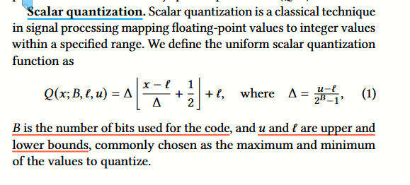
标量量化是一个非常古老的有损压缩算法。其核心是将一个 float 映射成一个固定位数的 int 整数,来减少向量每位的存储代价。
公式中的 B 是预计的量化空间,一般设置为 4 或者 8 ,代表我们将把 float 压缩成为 4bits or 8bits 来存储。
公式中的 Q 最后为下界 l 与一个量化结果的加和,实际存储中,下界 l 是全局共享的,因此只需要存储一次,前置的乘积即为量化结果,也就是每位都需要存储的 B bits 数据。
delta 指的是将单维的上下界平均分为 B bits 能够表示的若干份,每份是多大。因此 x - t / delta 便得到了 float x 比下界多了多少份,这是一个浮点数,可能多了 1.4 或者 1.5 份。如果直接向下取整,这两个都将被量化为 1 ,因此量化误差的所属区间便是 [0,1) 。
这里便出现了一个问题,我们拿 8 bits 量化举例:量化结果 0 对应的量化误差的所属区间是 **[0,1)**,因为 0 - 0.999…… 都会被量化至 0 ,但是量化结果为 2^8 - 1 的量化误差却变成了 0 ,也就是没有误差,原因是只有 2^8 - 1 会被量化至 2^8 - 1 。使用一个相同量化函数的量化结果,其误差率却不同,这代表我们的均匀函数是无法逻辑闭环的。
因此这个 0.5 的作用便清晰了,加了 0.5 ,任何量化结果都会有一段误差区间, 0 的量化误差区间便是 [0, 0.5) , 2^8 - 1 的量化误差区间便是 (-0.5, 0] 。加了一个 0.5 ,让每个量化结果都有一段属于它的 input。
同时,我们上述的 u l 两个边界,一般都是随机选取得到的,因此会出现一部分越界情况, 0.5 也允许部分越界的情况出现,增加了总体量化范围。如 不加 0.5 时, 0-127 能够表示的范围是 **[0, 127 * delta]**,而加了 0.5 ,能表示 [-0.5 * delta, 127.5 * delta]
为啥需要 0.5 ,简单解释: https://wu3227834.github.io/2024/02/18/2024-02-19-scalar-quantization/
二、LVQ - 局部自适应量化
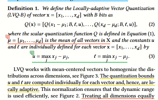
LVQ 是一个基于全局标量量化的量化算法,如上图所示的核心压缩算法所示。
其压缩算法的主要流程为:
1、遍历数据集,计算每个维度的均值,汇总为一个向量$$\mu$$
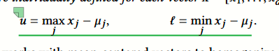
2、对于每个向量 x ,计算$$x - \mu$$,然后取其中的单维最大最小值为向量 x 的偏差上下界 u 和 l
3、将 $$x - \mu$$ 中的每个维度作为标量量化的待量化 float x 带入到标量量化公式中,将 向量x 的偏差上下界 u 和 l 作为标量量化的量化区间上下界带入到标量量化公式中,将目标量化 bit 数 B 代入,得到每个维度的量化结果。拼接得到整个向量的量化结果。
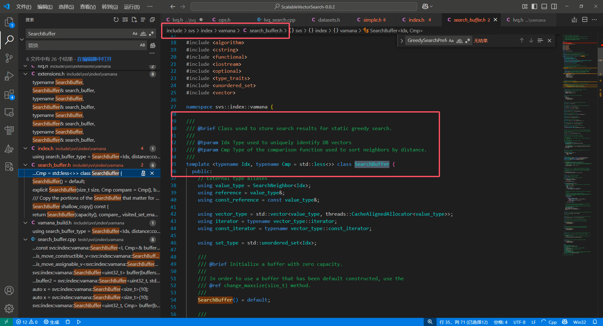
为了避免仅阅读论文导致的理解误差,我们需要阅读其源码:
LVQ 的官方指导文档:https://intel.github.io/ScalableVectorSearch/cpp/quantization/lvq.html#cpp-quantization-lvq
https://github.com/intel/ScalableVectorSearch/releases/tag/v0.0.2
由于 class LVQDataset 在后续版本中被迭代掉了,所以为了简单,我们选用了 v0.0.2 版本的源码进行阅读,核心代码如下图:
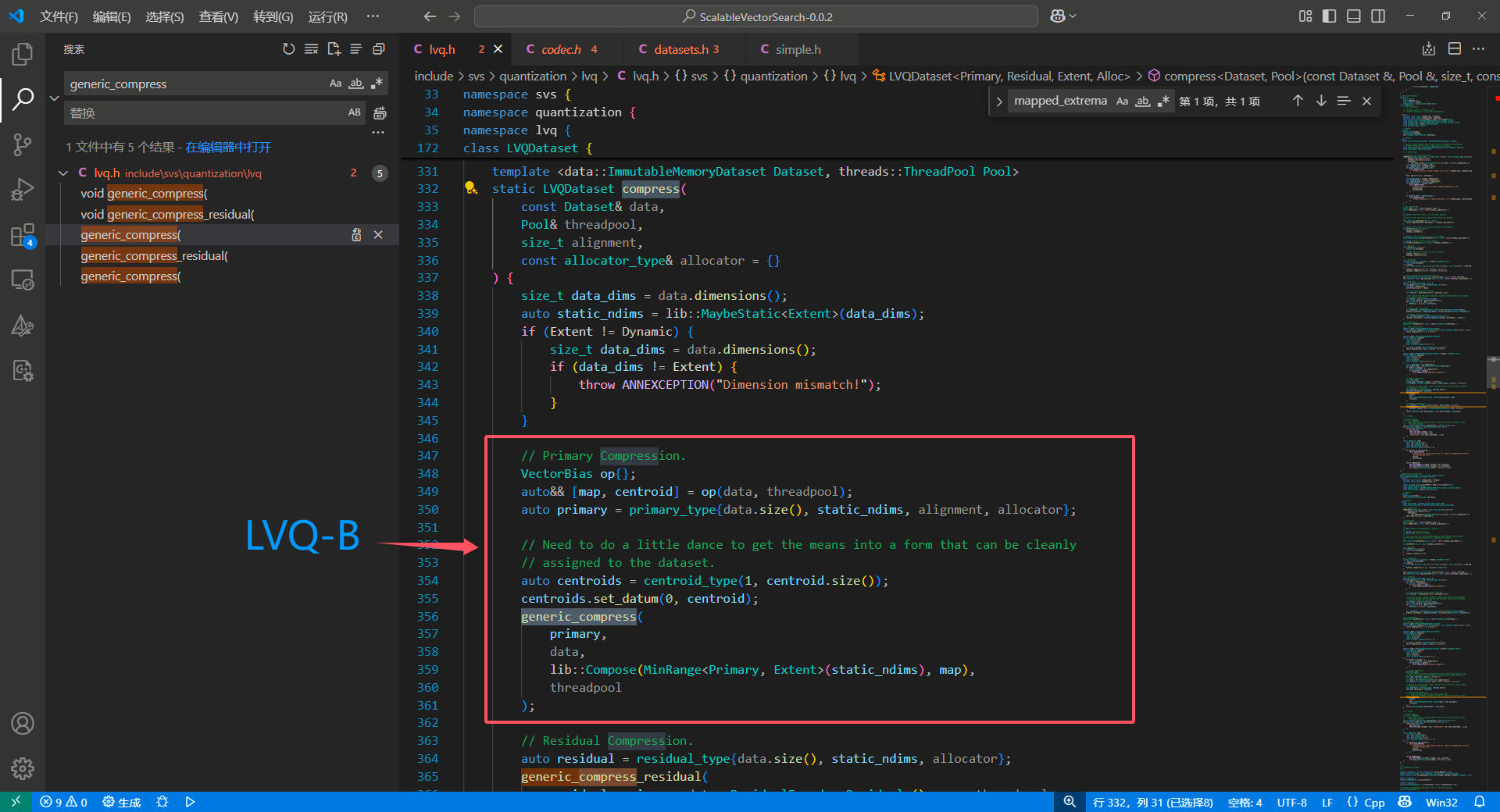
1、全局均值
1 | /// |
ScaleShift 是一个偏移量运算器, one 是偏移量运算后的缩放,在代码中通过
1 | auto ones = std::vector<double>(negative_means.size(), 1.0); |
设置为 1 ,也就是不额外缩放,因此 VectorBias() 实际上就是一个构造函数,返回了数据集 data 的
1、对同类型向量的异步去均值操作符 ScaleShift() ,将返回输入向量减去均值的结果,也就是我们上面算法中提到的 $$x - \mu$$
2、全局均值向量,也就是上面提到的 $$\mu$$
2、压缩运算符
level 1 压缩算法调用了压缩运算符,把输入的 raw data 压缩:
压缩运算符的具体实现如下:
1 |
|
这里的形式参数 data 是一个原始向量每个维度减去均值后的向量,也就是调用之前的 ScaleShift 函数后的结果,因此:
1 | auto [min, max] = extrema(data); |
实际上就是论文中的:
读到这里,我们便确定了理解的正确性。
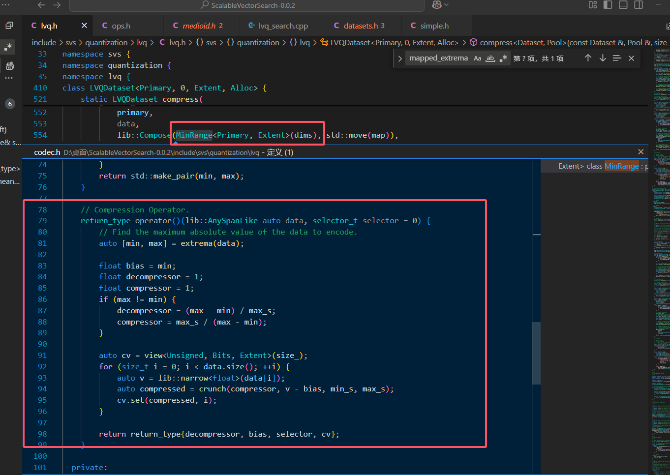
三、两阶段量化优化 - 最小化精度损失
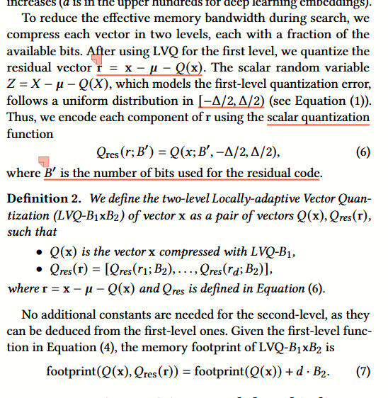
第一阶段的量化结果会出现精度损失,这部分损失实际上受到向量自身特性影响,如果一个向量有两个维度偏离均值很大,分别为 -10000 和 +10000 ,那么用 8bit 表示这个量化区间就会出现很大的精度问题。
因此,论文提出了第二阶段量化的概念,也就是把一阶段的量化精度误差作为 input ,比如刚刚的使用 8bit 量化区间 [-10000, +10000],那么数据便有 20000 / 127 = 157 的精度误差,因此,把这段误差再次使用 LVQ 进行量化,再解码时候把这部分数据加回去,便能够减少很多的误差。
(为了简便,这里的精度误差实际上应该是 [-(157/2), +(157/2)],正如论文中的正负二分之一 delta)
为了避免理解问题,我们再次去阅读下源码,源码中的具体实现如下图:
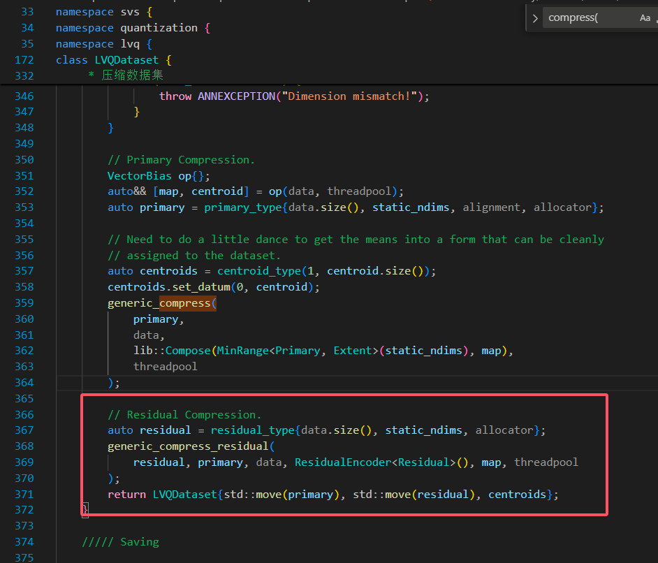
可以看到,和我们理解的并没有错误, primary 是一级压缩 LVQ-B 的量化结果,data 是原始向量。
上图中画圈部分是原始向量减去均值的向量,也就是一级压缩的实际参数,也就是论文中的:

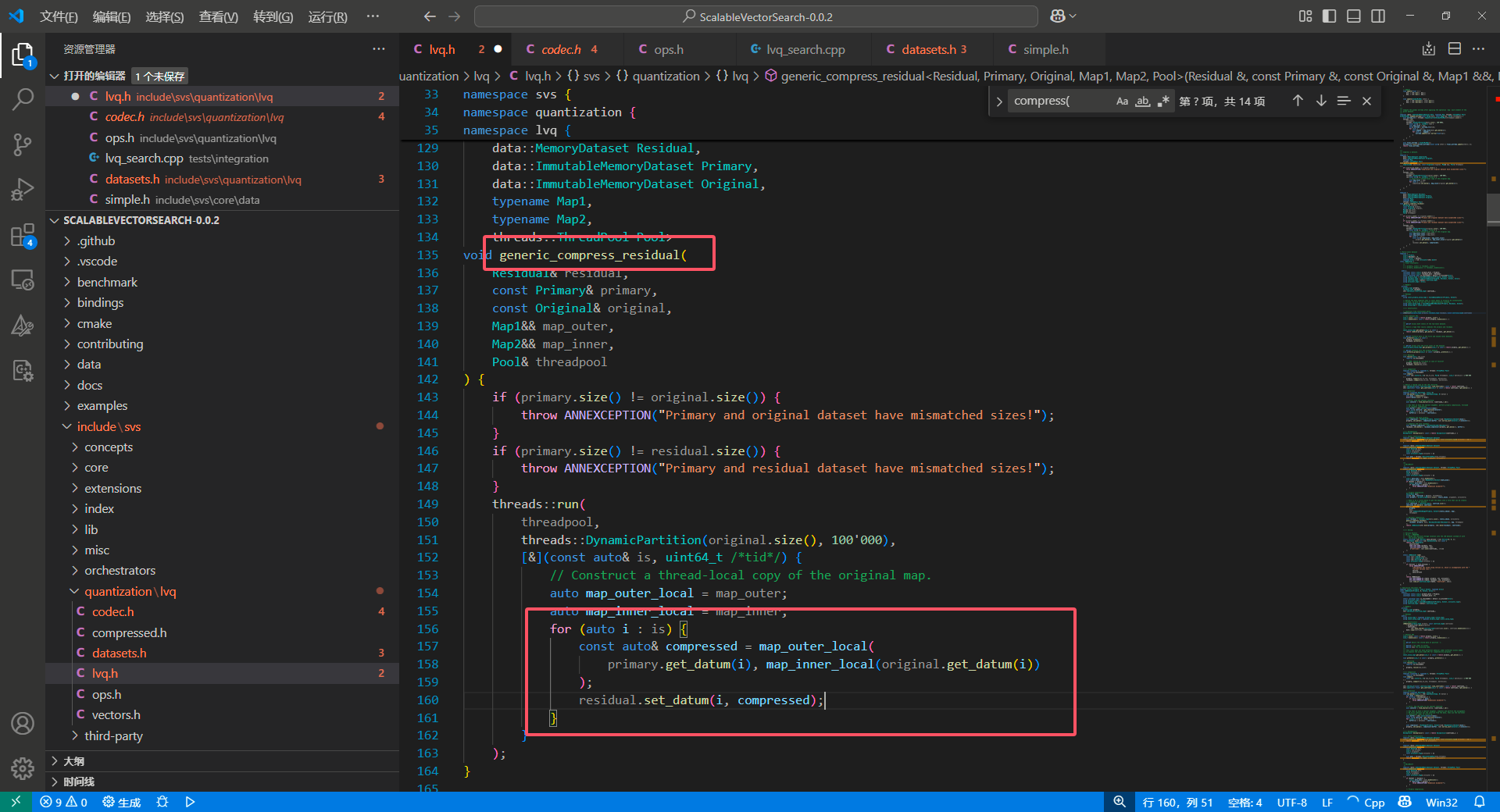
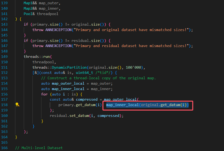
接着用它减去量化结果,也就是 primary 的对应数据,就得到了残差 residual ,接着用 ResidualEncoder 对其压缩即可。
ResidualEncoder 的具体实现位于:\ScalableVectorSearch-0.0.2\include\svs\quantization\lvq\codec.h ,这里我们不继续展开阅读了
图基索引应用
一、索引构建
LVQ 这篇论文的图基向量索引几乎是 DiskANN 的复制版本,也是用了一遍随机图
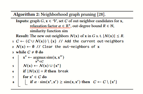
在裁边过程中,
二、选边的误差边界
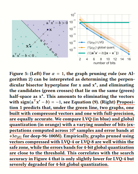
我们这里就不细致地阅读理论证明了,我们可以看右侧这幅图,绿色线是可用的理论边界 error 率。绿线下的都是在裁边时候可用的量化标准,可以看到 LVQ-4 比全局的 4bits 标量量化准确了很多。
三、对候选队列的影响
论文采用了 Ranked Bias Overlap (RBO) 作为指标,比较两个队列的相似度:
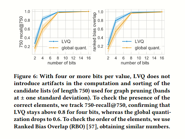
结果是在 8bits 以上的量化标准中,RBO 几乎一致,也就是说对查询几乎没有负面影响。
实现难题
这个章节是论文中比较有价值的地方,它尝试系统地描述,如何尽可能地优化一个 graph based 索引的性能。
一、Efcient similarity calculations using LVQ with AVX
1、利用 SIMD 进行计算加速,批量展开多个维度的数据,并计算距离
2、静态编译优化,让向量维度变为固定的,这一点很难在数据库中实现,但是对于固定维度的某些算法平台来说是可行的。
一些相关资料
https://www.zhihu.com/tardis/zm/art/409973153?source_id=1003
二、Advanced prefetching
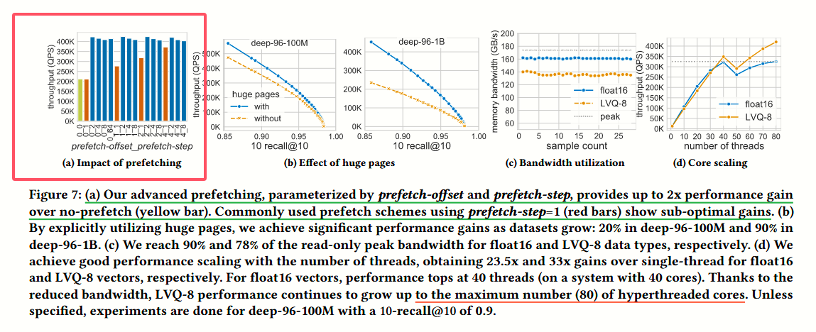
prefetch 是一项提前把可能短期访问的数据加载至 CPU cache 的技术,其实现可以分为硬件实现和软件实现,我们更关注的是软件实现。
其具体实现位于:
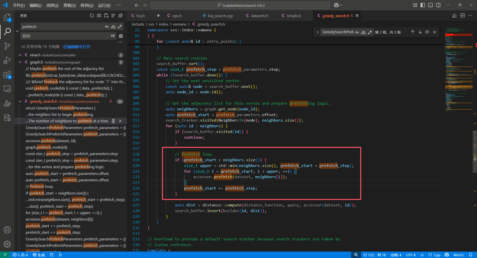
可以看到 software prefetch 的实现其实还是很简单的,但是这里提出的参数 0 和 2 是值得借鉴和实验的。
software prefetch 也在 hnswlib 中实现了,我们之前的实验中,software prefetch 也明显的提升了 hnswlib 的查询性能。
三、Optimizing graph search
1、排序算法优化
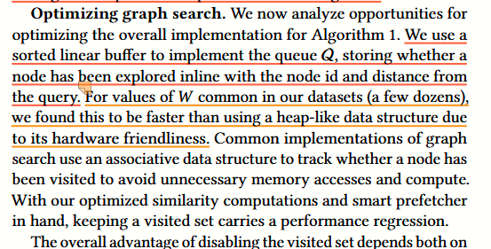
LVQ 的实现中,将全部的查询中间操作都封装进了一个名为 Buffer 的 type ,作者团队认为在 W 较小的时候,线性扫描的性能是优于堆排序的。
一个具体的实现是 SearchBuffer :
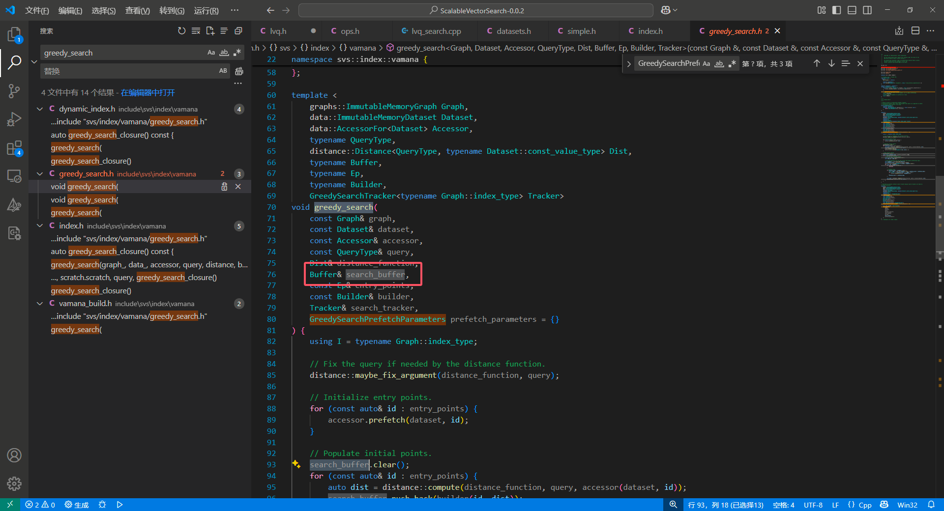
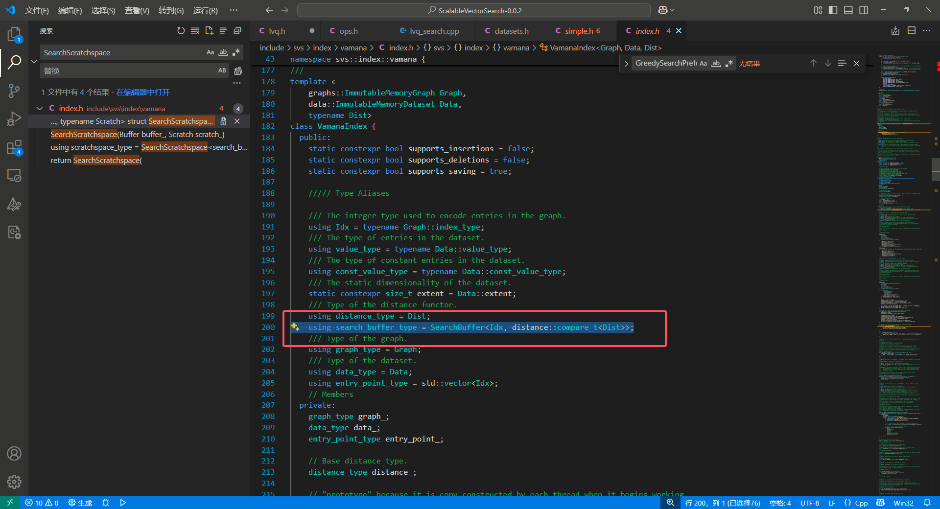
我们看一眼调用:
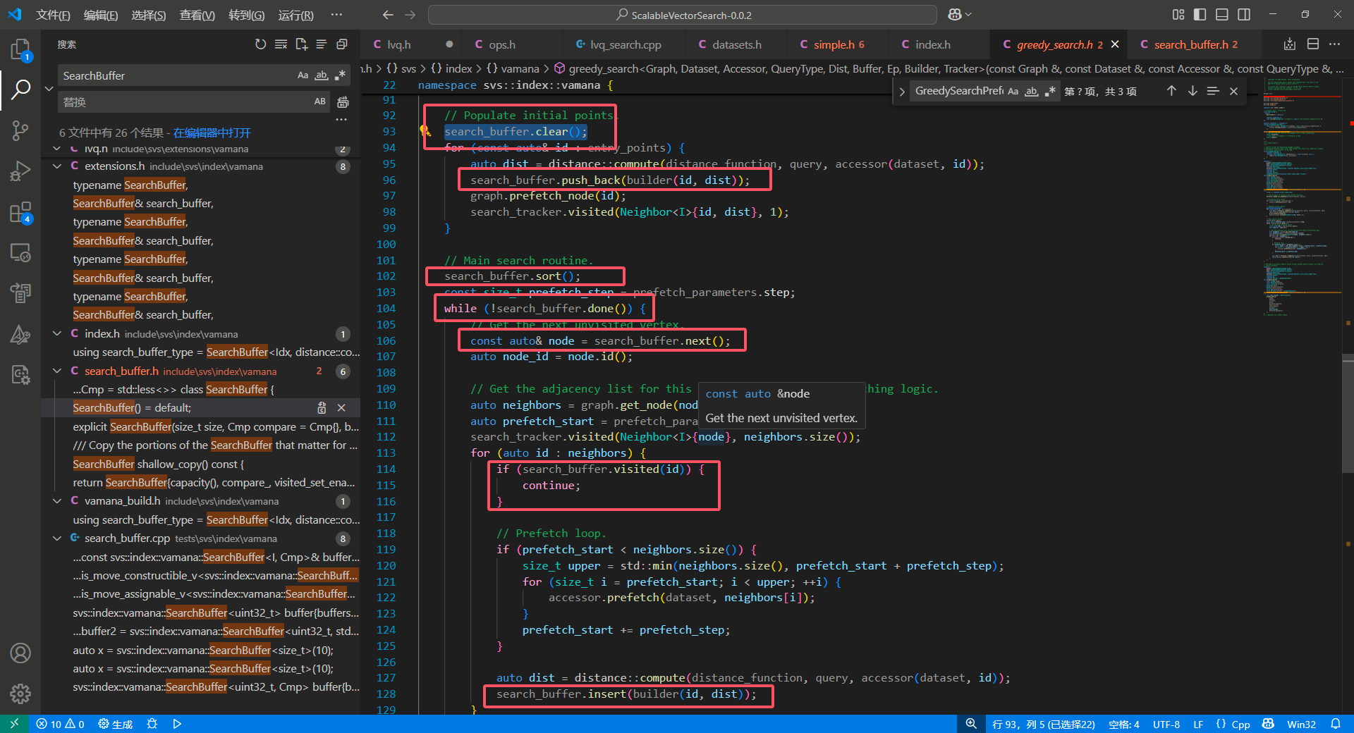
核心函数有几个:
1、sort

2、insert

3、visited

4、push_back
insert 函数是一个 copy 插入操作,调用了下面的 insert_inner ,其核心思想是从尾部顺序遍历,找到待插入位置,然后移动后面的数据,将数据插入到目标位置。
1 | size_t insert_inner(value_type neighbor) { |
我们可以看到,这个插入函数在大量数据会被尾插(仅仅在最后一个元素中更新)时表现的性能,可能会优于堆排。
2、visited hash set
我们可以回忆起 hnswlib 中的 visited hash 是通过全局直接映射实现的,但是这种实现方式的内存消耗有点大。使用局部 hashset 是一个可行的替代方案,但是 visited hash 的维护事实上有不小的消耗。
因此论文中决定取消掉 visited hash set ,通过与 candidate 耦合的 visited 标记 和一个动态的指向排序列表最后一个没有被访问的 candidate 的 best_unvisited_ 来实现这个功能:
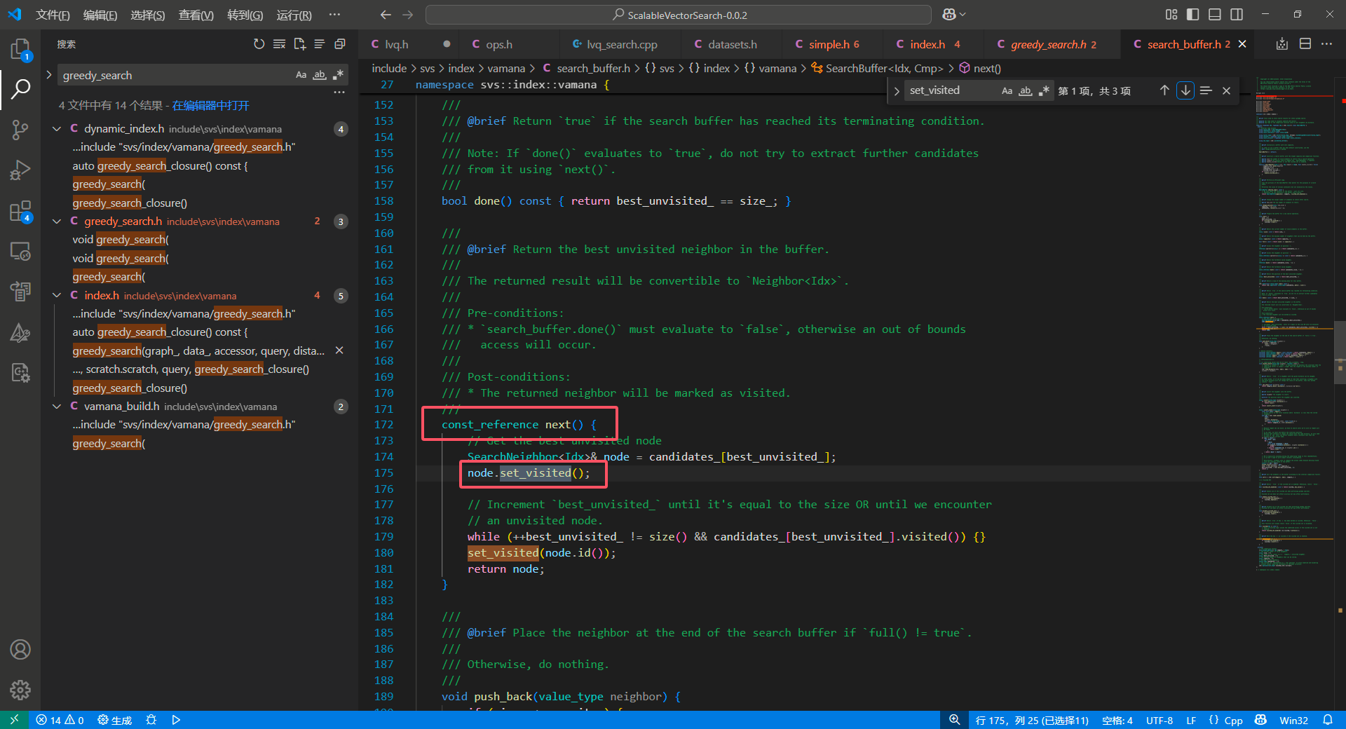
1 | // We're explicitly avoiding moving the underlying range in this implementaion, |
TODO: 这个优化的原理还需要再思考下,似乎是因为 hash 映射和维护是在 相似度计算&prefetch 之间的操作,可能会破坏 prefetch 的效果,把本来 load 进内存的数据驱逐掉。
四、Memory layout and allocation
这段主要是描述了 LVQ 利用 huge page 减少 TLB MISS 的优化,实验结果如下:
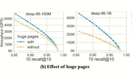
这里的优化原理还不是理解的很清晰,需要学习下
相关论文:Trident: Harnessing Architectural Resources for All Page Sizes in X86 Processors
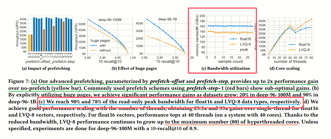
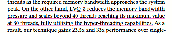
五、System utilization
这章节没什么好说的,主要是从 memory bandwidth 和 并发能力描述了 LVQ 的优点,也就是降低 内存带宽占用、并发性能优化。
实验
实验部分比较有意思的是消融实验:
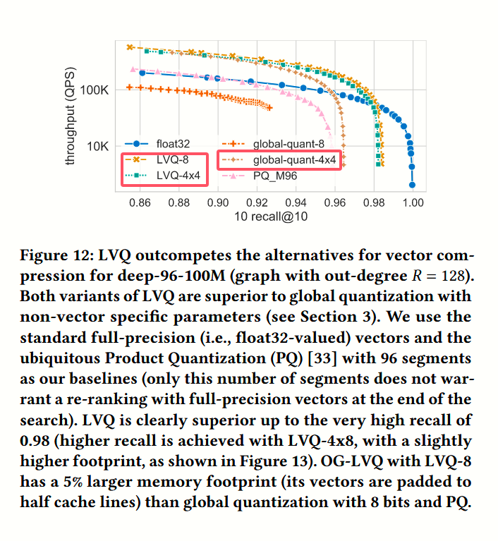
论文还额外地设计了 标量量化 + 4x4 的压缩实验,但是似乎没有进一步描述是怎样实现的。
思考
LVQ 是一篇 23 年的标量量化思想的压缩算法,并针对 vamana 图进行了一系列的优化手段。
这篇论文对我们的价值主要在
1、量化模型简单、2 层量化思想很有趣
2、prefetch 的实验设计有借鉴价值,尤其是 (0,2) 的 prefetch 参数设计
3、一些优化手段是值得我们借鉴的

